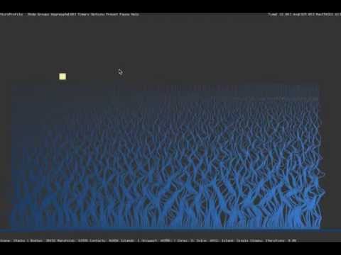
2D physics engine with SoA/SIMD optimizations
PhyX
Overview
This is a 2D physics engine with SoA/SIMD/multicore optimizations. The primary purpose of this project is to experiment with various multi-threading and SIMD algorithms - it is not meant to be a production-ready 2D physics engine.
The engine is based on SusliX by Alexander Sannikov aka Suslik <i.make.physics at gmail.com>
The optimizations are implemented by Arseny Kapoulkine <[email protected]>
The code is licensed under the MIT license.
Video
Building
To build the project, you first have to clone it using --recursive option to fetch the microprofile submodule.
On Linux/Mac, use make to build the project, and make run to run the demo. Makefile automatically picks the optimal compilation settings for the host system, using AVX2/FMA as appropriate.
On Windows, open phyx.sln in Visual Studio 2017 and build & run from there. Note that the project file is configured to assume AVX2 support; if your system doesn’t have AVX2, you will need to disable it by removing __AVX2__ from preprocessor defines and switching the code generation instruction set to “Streaming SIMD Extensions 2 (/arch:SSE2)” - both modifications can be done in project properties.
Features
The engine implements a traditional physics pipeline - broadphase, narrowphase, contact pairing/caching, island splitting, solve (using sequential impulses).
There is only one collision primitive - box. It should be straightforward to add support for more primitives, as long as each manifold has a small number of contact points.
There is only one constraint type - contact. It should be possible to add support for more constraint types, although that might require extensive changes to some algorithms, in particular SIMD.
The broadphase algorithm is single-axis sweep&prune, using non-incremental 3-pass radix sort. Incremental algorithms tend to be expensive when a lot of updates are performed, and sweep&prune is a good fit for 2D assuming the worlds are mostly horizontal.
Controls
In the demo you can use several keys to switch between various modes and cycle between scenes:
- Left/Right: move the viewport
- Up/Down: scale the viewport
- S: Switch to the next scene; different scenes test different configurations of bodies, stress testing various parts of the pipeline
- R: Reset current scene
- I: Switch island mode (see below)
- M: Switch solve mode (see below)
- C: Switch the number of cores the solver uses (1, 2, 4, 8, etc. - up to the number of logical core counts on the machine)
- P: Pause simulation
- O: Cycle between various microprofile display views
Island splitting
You can switch between different island construction modes by using the I key:
- Single: no island splitting is performed, constraint solving is effectively single-threaded.
- Multiple: objects are split into islands, each island is solved serially. Island splitting can be expensive for complex constraint graphs.
- Single Sloppy: no island splitting is performed, constraint solving is multi-threaded. Each internal solve step is serialized, which makes sure that - barring rare race conditions - impulse propagation is still effective.
- Multiple Sloppy: objects are split into islands, constraing solving within one island is multi-threaded. Compared to Single Sloppy, requires (potentially expensive) island splitting, but preserves mechanism integrity for small islands.
SIMD
The code is using a custom SIMD library and templated code that enables SIMD computations with both SSE2 (4-wide) and AVX2 (8-wide) with the same codebase. You can switch between different SIMD widths - 1, 4, 8 - using the M key.
The library interface is structured to make it easy to write complex algebraic code, including conditions:
Vf dv = -bounce * (relativeVelocityX * collision_normalX + relativeVelocityY * collision_normalY);
Vf depth = (point2X - point1X) * collision_normalX + (point2Y - point1Y) * collision_normalY;

Vf dstVelocity = max(dv - deltaVelocity, Vf::zero());

Vf j_normalLimiter_dstVelocity = select(dstVelocity, dstVelocity - maxPenetrationVelocity, depth < deltaDepth);
Vf j_normalLimiter_dstDisplacingVelocity = errorReduction * max(Vf::zero(), depth - Vf::one(2.0f) * deltaDepth);
Vf j_normalLimiter_accumulatedDisplacingImpulse = Vf::zero();
To be able to efficiently use SIMD, we split islands into groups of N independent constraints (that affect 2*N bodies), where N is the SIMD width. The constraint data is packed into AoSoA arrays (array of structure of arrays), otherwise known as block SoA where the block size matches SIMD width and each field of each vector is scalarized so that we can efficiently load and store them without a need to transpose. This structure is maintained throughout all internal iterations of the solver.
Threading
The code is using a pretty standard thread pool implementation with a single queue for items. This thread pool is used for distributing work across worker threads - the batches of work are very large to compensate for the inefficiency of locking/notification mechanisms, for example “one island” or “all contact points”.
On top of that we implement a parallelFor primitive that uses a shared atomic variable to concurrently process a large array of items. To reduce contention for the shared atomic, the arrays are split into small groups for batched processing. The code for using parallel for looks like this:
parallelFor(queue, 0, jointEnd - jointBegin, 128, [&](int i, int) {
    ContactJoint& joint = contactJoints[joint_index[jointBegin + i]];

    ContactJointPacked<N>& jointP = joint_packed[unsigned(jointBegin + i) / N];
    int iP = i & (N - 1);

    jointP.body1Index[iP] = joint.body1Index;
    jointP.body2Index[iP] = joint.body2Index;
    jointP.contactPointIndex[iP] = joint.contactPointIndex;

    jointP.normalLimiter_accumulatedImpulse[iP] = joint.normalLimiter_accumulatedImpulse;
    jointP.frictionLimiter_accumulatedImpulse[iP] = joint.frictionLimiter_accumulatedImpulse;
});
A bit of care is required to find optimal group size for each for loop; additionally, for small arrays it might be worthwhile to implement a serial path - although in case of the code above, parallelFor automatically serializes execution if there is only one group - that is, if the number of joints (jointEnd - jointBegin) is less than or equal to 128.
